R Tutorial : Multiple Linear Regression

This tutorial goes one step ahead from 2 variable regression to another type of regression which is Multiple Linear Regression. We will go through multiple linear regression using an example in R

Please also read though following Tutorials to get more familiarity on R and Linear regression background.

R : Basic Data Analysis – Part 1

R Tutorial : Intermediate Data Analysis – Part 2

Tutorial : Concept of Linearity in Linear Regression

Tutorial : Linear Regression Construct

R Tutorial : Basic 2 variable Linear Regression

Technique : Multiple Linear Regression

When to use : When our output variable is numeric

No of variables : > 2

Model Readability : High

For this tutorial we will be using csv version of the excel file uploaded here demandformoney. As always please save the file and then convert it to .csv using save as from excel.

Problem Statement

Central Bank prints paper money each year. For each year they need an estimate of how much money to be printed. The decision is based on various economic indicators like GDP, Interest rate etc. We will try to model the solution to this problem using Multiple linear regression.

Step 1 : Read File

money = read.csv("demandformoney.csv")
str(money)

‘data.frame’: 35 obs. of 5 variables:
$ year : int 1970 1971 1972 1973 1974 1975 1976 1977 1978 1979 …
$ Money_printed: int 7374 8323 9700 11200 11975 13325 16024 14388 17292 20000 …
$ GDP : int 474131 478918 477392 499120 504914 550379 557258 598885 631839 598974 …
$ Interest_RATE: num 7.25 7.25 7.25 7.25 9 10 10 9 9 10 …
$ WPI : num 14.3 15.1 16.7 20.1 25.1 24.8 25.3 26.6 26.6 31.2 …

Note : We have 4 variables of interest here Money_printed, GDP , Interest_RATE and WPI and we have conveniently omitted the variable year for a reason. But we will leave that discussion out for another tutorial post.

Step 2 : Identify the output variable and input variable

since ; 
Money_printed = f ( GDP , Interest_RATE , WPI )

output variable  : Money_printed

Input variables : GDP , Interest_RATE , WPI

Step 3 : Scatter plot

plot(money,col='red')

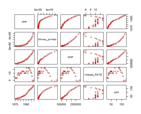
All the Input variables seem to be fairly linearly correlated with our output variable Money_printed except for WPI.

Step 4 : Construct a Linear model using R

multilinearmodel = lm (Money_printed ~ GDP + Interest_RATE + WPI, data = money)
summary(multilinearmodel)

Call:
lm(formula = Money_printed ~ GDP + Interest_RATE + WPI, data = money)

Residuals:
   Min     1Q Median     3Q    Max 
-46875  -7027   1387  15068  46249 

Coefficients:
                Estimate Std. Error t value Pr(>|t|)    
(Intercept)   -1.759e+04  5.052e+04  -0.348  0.73008    
GDP            2.975e-01  8.787e-02   3.385  0.00195 ** 
Interest_RATE -1.626e+04  2.919e+03  -5.570 4.19e-06 ***
WPI            2.943e+01  9.038e+02   0.033  0.97423    
---
Signif. codes:  0 ‘***’ 0.001 ‘**’ 0.01 ‘*’ 0.05 ‘.’ 0.1 ‘ ’ 1

Residual standard error: 22770 on 31 degrees of freedom
Multiple R-squared:  0.9848,	Adjusted R-squared:  0.9834 
F-statistic: 670.4 on 3 and 31 DF,  p-value: < 2.2e-16

Please note the formula used here is Money_printed ~ GDP + Interest_RATE + WPI
i.e Output Variable ~ Input Variable 1 + Input Variable 2 ….
An important point to be noted is the P value for variables GDP, Interest_RATE is significant i.e Pr(>|t|) for these variables is less than 0.05 .

For variable WPI however the P value is 0.97423 which is greater than 0.05 which is highly insignificant. What that means is that the variable WPI does not contribute significantly to the model and hence it must be removed.

Please also note that the Adjusted R Squared in 0.9834 which is fairly good but by removing an insignificant variable we can expect marginal increase in Adjusted R Squared as well.

Lets now go through another iteration of creating a model after omitting WPI from input variables.

multilinearmodel = lm (Money_printed ~ GDP + Interest_RATE , data = money)
summary(multilinearmodel)

Call:
lm(formula = Money_printed ~ GDP + Interest_RATE, data = money)

Residuals:
   Min     1Q Median     3Q    Max 
-47055  -7168   1432  14998  46008 

Coefficients:
                Estimate Std. Error t value Pr(>|t|)    
(Intercept)   -1.906e+04  2.192e+04  -0.870    0.391    
GDP            3.003e-01  6.913e-03  43.443  < 2e-16 ***
Interest_RATE -1.619e+04  1.977e+03  -8.191 2.35e-09 ***
---
Signif. codes:  0 ‘***’ 0.001 ‘**’ 0.01 ‘*’ 0.05 ‘.’ 0.1 ‘ ’ 1

Residual standard error: 22420 on 32 degrees of freedom
Multiple R-squared:  0.9848,	Adjusted R-squared:  0.9839 
F-statistic:  1038 on 2 and 32 DF,  p-value: < 2.2e-16

In this 2nd model please note that P values of both input variables are less than 0.05 and so both are significant variables for the model.
Also please note that Adjusted R Squared value has increased from 0.9834 to 0.9839 which is marginal increase but it still indicates that removing variable actually benefited our model.

We must ideally also consider distribution of our residuals before finalizing the model. But we will ignore this point now and accept the model since it has acceptable Adjusted R Squared.

Step 5 : Interpretation of output

From the coefficients of variables in the output above we construct our model for predicting Money_printed as –

Money_printed  = -19060 + 0.3003 * GDP – 16190 * Interest_RATE

Now when Central Bank needs to find how much Money is to be printed , they can plug in the values of GDP and Interest Rate into the equation above and find an estimate of money to be printed.

But before concluding that the model is good we must go through Residual Analysis , look at Adjusted R Squared values and interpret the F Statistic.

Hope you liked the post. Please post your reviews and comments and don’t forget to share.

Further you can read following tutorials for gaining further understanding

R Tutorial : Residual Analysis for Regression

R Tutorial : How to use Diagnostic Plots for Regression Models